Lecture 22 · November 5, 2026
Lecture reference
- Scales
- A scale maps a data domain to a visual range. Inputs can be quantitative, temporal, or categorical. Outputs can be position, length, radius, area, or color.
- Linear
y = r0 + (x − d0) / (d1 − d0) × (r1 − r0). A download of 400 MB out of 1600 MB maps to 2.5 inches out of 10. Constructor form:d3.scaleLinear([0, 1600], [0, 10]).- Scale families
- Linear, power, log, and symlog map continuous quantities. Time maps dates. Sequential and diverging scales interpolate colors. Quantile, quantize, and threshold produce discrete outputs. Ordinal maps categories to discrete values; band and point place categories along a continuous range.
- Axes
- Append an axis to an SVG group. D3 creates a domain path, tick groups, tick lines, and text labels. Translate the group to place the axis, rotate labels when needed, and use tick size to create grid lines.
- Encodings
- Marks include circles, lines, paths, rectangles, and text. Position, size, fill, opacity, stroke, and orientation can encode data.
- Chart families
- Bars, lines and areas, radial charts, dots, geospatial charts, hierarchies, and networks. D3 gallery ↗
01Mapping data with scales
async function build() {
  const svg = d3.select("#chart").append("svg")
      .attr("viewBox", "0 0 2000 1200")
      .attr("class", "scale-overview")
      .attr("width", 2000)
      .attr("height", 1200)
      .style("background", "#222");

  // Function to add section titles inside each group
  const addTitle = (group, text, x, y, fontSize) => {
      group.append("text")
          .attr("x", x)
          .attr("y", y)
          .attr("font-size", fontSize)
          .attr("fill", "white")
          .attr("font-weight", "bold")
          .text(text);
  };

  // 1. Linear Scale - Temperature Bars
  const linearGroup = svg.append("g").attr("transform", "translate(100, 50)");
  addTitle(linearGroup, "Linear Scale (Temperature → Rectangle Height)", 0, 0, 24);

  const tempScale = d3.scaleLinear().domain([0, 100]).range([10, 200]);
  const temperatures = [32, 45, 60, 75, 90, 100];

  linearGroup.selectAll(".temp-bars")
      .data(temperatures)
      .enter()
      .append("rect")
      .attr("x", (d, i) => i * 120)
      .attr("y", d => 50 + (200 - tempScale(d)))
      .attr("width", 60)
      .attr("height", d => tempScale(d))
      .attr("fill", "steelblue")
      .style("stroke", "#fff")
      .style("stroke-width", 2);


  // 2. Linear vs Sqrt Scale - Comparing Circle Sizes
  const circleGroup = svg.append("g").attr("transform", "translate(900, 50)");
  addTitle(circleGroup, "Comparing Linear vs Sqrt Scale (Value → Circle Radius)", 0, 0, 24);

  const linearRadiusScale = d3.scaleLinear().domain([1, 100]).range([5, 40]);
  const sqrtRadiusScale = d3.scaleSqrt().domain([1, 100]).range([5, 40]);
  const values = [1, 5, 10, 20, 50, 100];

  // Circles with scaleLinear()
  circleGroup.selectAll(".linear-circles")
      .data(values)
      .enter()
      .append("circle")
      .attr("cx", (d, i) => i * 150)
      .attr("cy", 120)
      .attr("r", d => linearRadiusScale(d))
      .attr("fill", "tomato")
      .style("stroke", "#fff")
      .style("stroke-width", 2);

  // Circles with scaleSqrt()
  circleGroup.selectAll(".sqrt-circles")
      .data(values)
      .enter()
      .append("circle")
      .attr("cx", (d, i) => i * 150)
      .attr("cy", 200)
      .attr("r", d => sqrtRadiusScale(d))
      .attr("fill", "orange")
      .style("stroke", "#fff")
      .style("stroke-width", 2);

  // 3. Band Scale - Vehicle Types
  const bandGroup = svg.append("g").attr("transform", "translate(100, 400)");
  addTitle(bandGroup, "Band Scale (Vehicle Types → Evenly Spaced Bars)", 0, 0, 24);

  const vehicles = ["Sedan", "SUV", "Truck", "Motorcycle", "Electric"];
  const vehicleScale = d3.scaleBand().domain(vehicles).range([0, 600]).padding(0.2);

  bandGroup.selectAll(".vehicle-bars")
      .data(vehicles)
      .enter()
      .append("rect")
      .attr("x", d => vehicleScale(d))
      .attr("y", 50)
      .attr("width", vehicleScale.bandwidth())
      .attr("height", 50)
      .attr("fill", "darkorange")
      .style("stroke", "#fff")
      .style("stroke-width", 2);

  bandGroup.selectAll(".vehicle-labels")
      .data(vehicles)
      .enter()
      .append("text")
      .attr("x", d => vehicleScale(d) + vehicleScale.bandwidth() / 2)
      .attr("y", 80)
      .attr("text-anchor", "middle")
      .attr("fill", "white")
      .attr("font-size", "16px")
      .text(d => d);

  // 4. Time Scale - Timeline Events
  const timeGroup = svg.append("g").attr("transform", "translate(900, 400)");
  addTitle(timeGroup, "Time Scale (Events → Timeline)", 0, 0, 24);

  const eventScale = d3.scaleTime()
      .domain([new Date("2000-07-01"), new Date("2030-07-01")])
      .range([0, 600]);

  const events = [
      { year: new Date("2005-07-01") },
      { year: new Date("2010-07-01") },
      { year: new Date("2015-07-01") },
      { year: new Date("2020-07-01") },
      { year: new Date("2025-07-01") }
  ];

  // Draw event lines
  timeGroup.selectAll(".timeline-events")
      .data(events)
      .enter()
      .append("line")
      .attr("x1", d => eventScale(d.year))
      .attr("x2", d => eventScale(d.year))
      .attr("y1", 50)
      .attr("y2", 100)
      .style("stroke", "white")
      .style("stroke-width", 2);

  // Format date as "YYYY"
  const formatDate = d3.timeFormat("%Y");

  timeGroup.selectAll(".timeline-labels")
      .data(events)
      .enter()
      .append("text")
      .attr("x", d => eventScale(d.year))
      .attr("y", 40)
      .attr("text-anchor", "middle") // Center text
      .attr("fill", "white")
      .attr("font-size", "16px")
      .text(d => formatDate(d.year));


  // 5. d3-scale-chromatic Color Scales
  const colorGroup = svg.append("g").attr("transform", "translate(100, 600)");
  addTitle(colorGroup, "D3-Scale-Chromatic", 0, 0, 24);

  const colorValues = d3.range(15);
  const divergingValues = d3.range(15);

  const ordinalScales = [
      { name: "Category10", scale: d3.scaleOrdinal(d3.schemeCategory10) },
      { name: "Tableau10", scale: d3.scaleOrdinal(d3.schemeTableau10) }
  ];

  const sequentialScales = [
      { name: "Blues", scale: d3.scaleSequential(d3.interpolateBlues).domain([0, 14]) },
      { name: "Viridis", scale: d3.scaleSequential(d3.interpolateViridis).domain([0, 14]) }
  ];

  const divergingScales = [
      { name: "RdYlBu", scale: d3.scaleDiverging(d3.interpolateRdYlBu).domain([0, 7, 14]) }, // you need to add midpoint value for diverging scale!
      { name: "PuOr", scale: d3.scaleDiverging(d3.interpolatePuOr).domain([0, 7, 14]) }
  ];

  const drawColorScaleGroup = (group, scales, startX, startY, values) => {
      scales.forEach((colorScheme, rowIndex) => {
          const rowY = startY + rowIndex * 50;

          group.append("text")
              .attr("x", startX - 120)
              .attr("y", rowY + 25)
              .attr("text-anchor", "start")
              .attr("fill", "white")
              .attr("font-size", "18px")
              .text(colorScheme.name);

          // Draw a row of color-filled rectangles
          group.selectAll(`.color-bar-${colorScheme.name}`)
              .data(values)
              .enter()
              .append("rect")
              .attr("x", (d, i) => startX + i * 25)
              .attr("y", rowY)
              .attr("width", 23)
              .attr("height", 35)
              .attr("fill", d => colorScheme.scale(d))
              .style("stroke", "#fff")
              .style("stroke-width", 1);
      });
  };

  const ordinalGroup = colorGroup.append("g").attr("transform", "translate(0, 40)");
  addTitle(ordinalGroup, "Ordinal (Categorical) Scales", 0, -5);
  drawColorScaleGroup(ordinalGroup, ordinalScales, 100, 10, colorValues);

  const sequentialGroup = colorGroup.append("g").attr("transform", "translate(700, 40)");
  addTitle(sequentialGroup, "Sequential Scales", 0, -5);
  drawColorScaleGroup(sequentialGroup, sequentialScales, 100, 10, colorValues);

  const divergingGroup = colorGroup.append("g").attr("transform", "translate(100, 200)");
  addTitle(divergingGroup, "Diverging Scales", 0, -5);
  drawColorScaleGroup(divergingGroup, divergingScales, 100, 10, divergingValues);
}

build();
Data & source
Lecture 22, slides 2–12
The complete combined scales demonstration from the supplied D3 Scales tutorial, including vehicle bands, the event timeline, radius comparisons, and all color palettes.
02Scale types
async function build() {
  const W = 960, H = 560;
  const margin = {top: 42, right: 135, bottom: 90, left: 74};
  const w = W - margin.left - margin.right;
  const h = H - margin.top - margin.bottom;
  const svg = d3.select('#chart').append('svg')
    .attr('viewBox', `0 0 ${W} ${H}`).attr('role', 'img')
    .attr('aria-label', "Scale types");
  const plot = svg.append('g')
    .attr('transform', `translate(${margin.left},${margin.top})`);

  // Quantitative, temporal, and categorical domains use different mappings.
  const months = ['Jan', 'Feb', 'Mar', 'Jul', 'May', 'Jun', 'Jul', 'Aug', 'Sep', 'Oct', 'Nov', 'Dec'];
  const rows = [
    ['Linear', d3.scaleLinear().domain([0, 1600]).range([0, 10]), 400],
    ['Time', d3.scaleTime().domain([new Date('2000-01-01'), new Date('2001-01-01')]).range([1, 100]), new Date('2000-07-02')],
    ['Pow (exponent 2)', d3.scalePow().domain([0, 10]).range([0, 100]).exponent(2), 5],
    ['Sqrt', d3.scaleSqrt().domain([0, 100]).range([0, 100]), 25],
    ['Log', d3.scaleLog().domain([1, 1000]).range([0, 100]), 10],
    ['SymLog', d3.scaleSymlog().domain([-100, 100]).range([0, 100]), 0],
    ['Band', d3.scaleBand().domain(months).range([0, 1200]), 'Jul'],
    ['Point', d3.scalePoint().domain(months).range([0, 1200]), 'Jul'],
    ['Ordinal', d3.scaleOrdinal().domain(months).range(d3.schemeAccent), 'Jul'],
    ['Sequential', d3.scaleSequential(d3.interpolateBlues).domain([0, 100]), 75],
    ['Diverging', d3.scaleDiverging(d3.interpolateRdYlBu).domain([-1, 0, 1]), 0.5],
    ['Quantile', d3.scaleQuantile().domain([1, 2, 3, 4, 5, 30, 80, 100]).range(['low', 'middle', 'high']), 30],
    ['Quantize', d3.scaleQuantize().domain([0, 100]).range(['low', 'middle', 'high']), 30],
    ['Threshold', d3.scaleThreshold().domain([20, 50]).range(['low', 'middle', 'high']), 30]
  ];
  rows.forEach(([name, scale, input], i) => {
    const row = plot.append('g').attr('transform', `translate(0,${i * 30})`);
    row.append('text').attr('x', 0).attr('y', 16).text(name);
    const output = scale(input);
    row.append('text').attr('x', 190).attr('y', 16)
      .text(`${input instanceof Date ? d3.timeFormat('%Y-%m-%d')(input) : input} → ${typeof output === 'number' ? d3.format('.2f')(output) : output}`);
  });
  // A band occupies an interval; a point scale supplies only a position.
  console.log('Band width:', rows[6][1].bandwidth());
  console.log('400 / 1600 =', rows[0][1](400), 'inches out of 10');
}

build();
Data & source
Lecture 22, slides 2–8
03Linear and square-root radius
async function build() {
  const W = 960, H = 560;
  const margin = {top: 42, right: 135, bottom: 90, left: 74};
  const w = W - margin.left - margin.right;
  const h = H - margin.top - margin.bottom;
  const svg = d3.select('#chart').append('svg')
    .attr('viewBox', `0 0 ${W} ${H}`).attr('role', 'img')
    .attr('aria-label', "Linear and square-root radius");
  const plot = svg.append('g')
    .attr('transform', `translate(${margin.left},${margin.top})`);

  const values = [1, 5, 10, 20, 50, 100];
  const linear = d3.scaleLinear().domain([0, 100]).range([0, 46]);
  const sqrt = d3.scaleSqrt().domain([0, 100]).range([0, 46]);
  const x = d3.scalePoint().domain(values).range([70, w - 40]);
  [['Linear radius', linear, 110, 'tomato'], ['Square-root radius', sqrt, 265, 'orange']]
    .forEach(([name, radius, y, fill]) => {
      plot.append('text').attr('y', y - 65).text(name);
      plot.append('g').selectAll('circle').data(values).join('circle')
        .attr('cx', x).attr('cy', y).attr('r', radius).attr('fill', fill);
      plot.append('g').selectAll('text').data(values).join('text')
        .attr('x', x).attr('y', y + 65).attr('text-anchor', 'middle').text(d => d);
    });
  // A square-root radius makes circle area proportional to the data value.
}

build();
Data & source
Lecture 22, slides 7, 12
04Color schemes and interpolation
async function build() {
  const W = 960, H = 560;
  const margin = {top: 42, right: 135, bottom: 90, left: 74};
  const w = W - margin.left - margin.right;
  const h = H - margin.top - margin.bottom;
  const svg = d3.select('#chart').append('svg')
    .attr('viewBox', `0 0 ${W} ${H}`).attr('role', 'img')
    .attr('aria-label', "Color schemes and interpolation");
  const plot = svg.append('g')
    .attr('transform', `translate(${margin.left},${margin.top})`);

  const values = d3.range(15);
  const schemes = [
    ['Accent', d3.scaleOrdinal(d3.schemeAccent)],
    ['Category10', d3.scaleOrdinal(d3.schemeCategory10)],
    ['Tableau10', d3.scaleOrdinal(d3.schemeTableau10)],
    ['Blues', d3.scaleSequential(d3.interpolateBlues).domain([0, 14])],
    ['Viridis', d3.scaleSequential(d3.interpolateViridis).domain([0, 14])],
    ['RdYlBu', d3.scaleDiverging(d3.interpolateRdYlBu).domain([0, 7, 14])],
    ['PuOr', d3.scaleDiverging(d3.interpolatePuOr).domain([0, 7, 14])]
  ];
  schemes.forEach(([name, scale], row) => {
    const g = plot.append('g').attr('transform', `translate(0,${row * 42})`);
    g.append('text').attr('y', 21).text(name);
    g.selectAll('rect').data(values).join('rect')
      .attr('x', (d, i) => 110 + i * 35).attr('width', 33).attr('height', 30)
      .attr('fill', scale);
  });
  const color = d3.scaleLinear().domain([-1, 0, 1]).range(['red', 'white', 'green']);
  const pixels = d3.scaleLinear().domain([0, 1]).range(['20px', '36px']);
  plot.append('text').attr('y', 335).text(`Piecewise color(0.5): ${color(0.5)}`);
  plot.append('text').attr('y', 370).text(`String interpolation: pixels(0.5) = ${pixels(0.5)}`);
}

build();
Data & source
Lecture 22, slides 5, 9–12
05Axes and customization
async function build() {
  const W = 960, H = 560;
  const margin = {top: 42, right: 135, bottom: 90, left: 74};
  const w = W - margin.left - margin.right;
  const h = H - margin.top - margin.bottom;
  const svg = d3.select('#chart').append('svg')
    .attr('viewBox', `0 0 ${W} ${H}`).attr('role', 'img')
    .attr('aria-label', "Axes and customization");
  const plot = svg.append('g')
    .attr('transform', `translate(${margin.left},${margin.top})`);

  const x = d3.scaleLinear().domain([0, 100]).range([0, w]);
  const y = d3.scaleLinear().domain([0, 100]).range([h, 0]);
  const xAxis = d3.axisBottom(x).ticks(7).tickSizeInner(-h);
  const axisGroup = plot.append('g').attr('transform', `translate(0,${h})`).call(xAxis);
  axisGroup.selectAll('text').attr('transform', 'rotate(-45)').attr('text-anchor', 'end');
  axisGroup.selectAll('.tick line').attr('stroke', '#ddd');
  plot.append('g').call(d3.axisLeft(y).ticks(5));
  plot.append('g').call(d3.axisTop(x).ticks(7));
  plot.append('g').attr('transform', `translate(${w},0)`).call(d3.axisRight(y).ticks(5));
  const categories = ['Jan', 'Feb', 'Mar', 'Apr', 'May', 'Jun'];
  const band = d3.scaleBand().domain(categories).range([0, w]).padding(0.15);
  plot.append('g').attr('transform', `translate(0,${h / 2})`)
    .call(d3.axisBottom(band)).style('color', '#168b8e');
  // D3 generates a domain path and a <g class="tick"> for each tick.
  console.log(axisGroup.node().outerHTML);
}

build();
Data & source
Lecture 22, slides 13–17
06Marks and visual encodings
async function build() {
  const W = 960, H = 560;
  const margin = {top: 42, right: 135, bottom: 90, left: 74};
  const w = W - margin.left - margin.right;
  const h = H - margin.top - margin.bottom;
  const svg = d3.select('#chart').append('svg')
    .attr('viewBox', `0 0 ${W} ${H}`).attr('role', 'img')
    .attr('aria-label', "Marks and visual encodings");
  const plot = svg.append('g')
    .attr('transform', `translate(${margin.left},${margin.top})`);

  const data = [{value: 20, group: 'A'}, {value: 45, group: 'B'}, {value: 70, group: 'A'}, {value: 100, group: 'C'}];
  const x = d3.scaleLinear().domain([0, 100]).range([50, w - 70]);
  const radius = d3.scaleSqrt().domain([0, 100]).range([0, 34]);
  const color = d3.scaleOrdinal(d3.schemeAccent).domain(['A', 'B', 'C']);
  plot.selectAll('circle').data(data).join('circle')
    .attr('cx', d => x(d.value)).attr('cy', 65).attr('r', d => radius(d.value))
    .attr('fill', d => color(d.group)).attr('opacity', 0.8)
    .attr('stroke', '#e0e0e0').attr('stroke-width', 2);
  plot.selectAll('rect').data(data).join('rect')
    .attr('x', d => x(d.value) - 18).attr('y', d => 250 - d.value)
    .attr('width', 36).attr('height', d => d.value).attr('fill', d => color(d.group));
  plot.append('line').attr('x1', 20).attr('x2', w).attr('y1', 285).attr('y2', 285)
    .attr('stroke', '#e0e0e0').attr('stroke-width', 3).attr('stroke-dasharray', '8 5');
  plot.selectAll('text').data(data).join('text').attr('x', d => x(d.value)).attr('y', 330)
    .attr('text-anchor', 'middle').text(d => `${d.group}: ${d.value}`);
  // Circle radius, rectangle height, position, fill, opacity, and stroke encode data.
}

build();
Data & source
Lecture 22, slides 18–20
07Vertical bar chart
async function build() {
  const W = 960, H = 560;
  const margin = {top: 42, right: 135, bottom: 90, left: 74};
  const w = W - margin.left - margin.right;
  const h = H - margin.top - margin.bottom;
  const svg = d3.select('#chart').append('svg')
    .attr('viewBox', `0 0 ${W} ${H}`).attr('role', 'img')
    .attr('aria-label', "Vertical bar chart");
  const plot = svg.append('g')
    .attr('transform', `translate(${margin.left},${margin.top})`);

  const raw = await d3.csv('./examples/01_scales_axes_marks/datasets/colleges.csv', d3.autoType);
  const data = raw.filter(d => Number.isFinite(d['SAT Average']) && d.Name)
    .sort((a, b) => d3.descending(a['SAT Average'], b['SAT Average'])).slice(0, 100);
  const x = d3.scaleBand().domain(data.map(d => d.Name)).range([0, w]).paddingInner(0.1);
  const y = d3.scaleLinear().domain([0, d3.max(data, d => d['SAT Average'])]).nice().range([h, 0]);
  const color = d3.scaleOrdinal(d3.schemeCategory10).domain(data.map(d => d.Control));
  plot.selectAll('.bar').data(data).join('rect').attr('class', 'bar')
    .attr('x', d => x(d.Name)).attr('y', d => y(d['SAT Average']))
    .attr('width', x.bandwidth()).attr('height', d => h - y(d['SAT Average']))
    .attr('fill', d => color(d.Control))
    .append('title').text(d => `${d.Name}: ${d['SAT Average']}`);
  plot.append('g').attr('transform', `translate(0,${h})`)
    .call(d3.axisBottom(x).tickValues(x.domain().filter((d, i) => i % 10 === 0)))
    .selectAll('text').attr('transform', 'rotate(-45)').attr('text-anchor', 'end')
    .text(d => d.length > 17 ? d.slice(0, 16) + '…' : d);
  plot.append('g').call(d3.axisLeft(y).ticks(6));
  svg.append('text').attr('x', margin.left).attr('y', 23).text('Top 100 colleges by SAT average');
  const legend = svg.append('g').attr('transform', `translate(${W - 120},60)`);
  color.domain().forEach((control, i) => {
    legend.append('rect').attr('y', i * 25).attr('width', 12).attr('height', 12).attr('fill', color(control));
    legend.append('text').attr('x', 18).attr('y', i * 25 + 11).text(control);
  });
}

build();
Data & source
Lecture 22, slides 21–27
08Scatterplot
async function build() {
  const W = 960, H = 560;
  const margin = {top: 42, right: 135, bottom: 90, left: 74};
  const w = W - margin.left - margin.right;
  const h = H - margin.top - margin.bottom;
  const svg = d3.select('#chart').append('svg')
    .attr('viewBox', `0 0 ${W} ${H}`).attr('role', 'img')
    .attr('aria-label', "Scatterplot");
  const plot = svg.append('g')
    .attr('transform', `translate(${margin.left},${margin.top})`);

  const raw = await d3.csv('./examples/01_scales_axes_marks/datasets/colleges.csv', d3.autoType);
  const data = raw.filter(d => d['Undergrad Population'] > 0 && d['Average Cost'] > 0 && d.Control);
  const x = d3.scaleLinear().domain(d3.extent(data, d => d['Undergrad Population'])).nice().range([0, w]);
  const y = d3.scaleLinear().domain(d3.extent(data, d => d['Average Cost'])).nice().range([h, 0]);
  const color = d3.scaleOrdinal(d3.schemeCategory10).domain(data.map(d => d.Control));
  plot.append('g').attr('transform', `translate(0,${h})`)
    .call(d3.axisBottom(x).tickSize(-h).tickFormat('')).attr('opacity', 0.15);
  plot.append('g').call(d3.axisLeft(y).tickSize(-w).tickFormat('')).attr('opacity', 0.15);
  plot.selectAll('.college').data(data).join('circle').attr('class', 'college')
    .attr('cx', d => x(d['Undergrad Population'])).attr('cy', d => y(d['Average Cost']))
    .attr('r', 5).attr('fill', d => color(d.Control)).attr('opacity', 0.6)
    .append('title').text(d => d.Name);
  plot.append('g').attr('transform', `translate(0,${h})`).call(d3.axisBottom(x).ticks(6));
  plot.append('g').call(d3.axisLeft(y).ticks(6).tickFormat(d3.format('~s')));
  svg.append('text').attr('x', margin.left + w / 2).attr('y', H - 18).attr('text-anchor', 'middle').text('Undergraduate population');
  svg.append('text').attr('transform', `translate(18,${H / 2}) rotate(-90)`)
    .attr('text-anchor', 'middle').text('Average cost');
  const legend = svg.append('g').attr('transform', `translate(${W - 120},60)`);
  color.domain().forEach((control, i) => {
    legend.append('rect').attr('y', i * 25).attr('width', 12).attr('height', 12).attr('fill', color(control));
    legend.append('text').attr('x', 18).attr('y', i * 25 + 11).text(control);
  });
}

build();
Data & source
Lecture 22, slides 28–34
09SVG path commands
async function build() {
  const W = 960, H = 560;
  const margin = {top: 42, right: 135, bottom: 90, left: 74};
  const w = W - margin.left - margin.right;
  const h = H - margin.top - margin.bottom;
  const svg = d3.select('#chart').append('svg')
    .attr('viewBox', `0 0 ${W} ${H}`).attr('role', 'img')
    .attr('aria-label', "SVG path commands");
  const plot = svg.append('g')
    .attr('transform', `translate(${margin.left},${margin.top})`);

  // Uppercase commands use absolute coordinates; lowercase commands are relative.
  const paths = [
    ['M / L / Z', 'M70 15 L15 130 L125 130 Z'],
    ['H / V', 'M15 15 H125 V130 H15 Z'],
    ['C / S', 'M15 110 C15 10 70 10 70 70 S125 130 140 25'],
    ['Q / T', 'M15 110 Q70 0 125 110 T235 110'],
    ['A', 'M15 110 A60 45 0 0 1 135 110'],
    ['Relative l / q', 'M15 130 l60 -110 l60 110 M15 130 q60 -120 120 0']
  ];
  paths.forEach(([name, d], i) => {
    const g = plot.append('g').attr('transform', `translate(${(i % 3) * 235},${Math.floor(i / 3) * 195})`);
    g.append('text').attr('y', -5).text(name);
    g.append('path').attr('d', d).attr('fill', 'none')
      .attr('stroke', d3.schemeTableau10[i]).attr('stroke-width', 3);
  });
  // M move, L line, H horizontal, V vertical, C cubic Bézier, S smooth cubic,
  // Q quadratic Bézier, T smooth quadratic, A elliptical arc, Z close.
}

build();
Data & source
Lecture 22, slides 36–37
10Line generators and curves
async function build() {
  const W = 960, H = 560;
  const margin = {top: 42, right: 135, bottom: 90, left: 74};
  const w = W - margin.left - margin.right;
  const h = H - margin.top - margin.bottom;
  const svg = d3.select('#chart').append('svg')
    .attr('viewBox', `0 0 ${W} ${H}`).attr('role', 'img')
    .attr('aria-label', "Line generators and curves");
  const plot = svg.append('g')
    .attr('transform', `translate(${margin.left},${margin.top})`);

  const points = [[10, 60], [40, 90], [60, 10], [190, 10]];
  const path = d3.line()(points); // M10,60L40,90L60,10L190,10
  plot.append('text').attr('y', 15).text(path);
  const curves = [['Linear', d3.curveLinear], ['Basis', d3.curveBasis], ['Monotone X', d3.curveMonotoneX]];
  curves.forEach(([name, curve], i) => {
    const g = plot.append('g').attr('transform', `translate(${i * 235},100)`);
    const line = d3.line().curve(curve);
    g.append('path').datum(points).attr('d', line).attr('fill', 'none')
      .attr('stroke', d3.schemeTableau10[i]).attr('stroke-width', 3);
    g.selectAll('circle').data(points).join('circle').attr('cx', d => d[0])
      .attr('cy', d => d[1]).attr('r', 4).attr('fill', '#e0e0e0');
    g.append('text').attr('y', 150).text(name);
  });
  // datum binds one array to a path. data binds a collection to multiple marks.
}

build();
Data & source
Lecture 22, slides 38–40
11Population line chart
async function build() {
  const W = 960, H = 560;
  const margin = {top: 42, right: 135, bottom: 90, left: 74};
  const w = W - margin.left - margin.right;
  const h = H - margin.top - margin.bottom;
  const svg = d3.select('#chart').append('svg')
    .attr('viewBox', `0 0 ${W} ${H}`).attr('role', 'img')
    .attr('aria-label', "Population line chart");
  const plot = svg.append('g')
    .attr('transform', `translate(${margin.left},${margin.top})`);

  const raw = await d3.json('./examples/02_advanced_charts/datasets/population.json');
  const data = raw.map(d => ({...d, sex: d.sex === 1 ? 'male' : 'female', year: new Date(d.year, 0, 1)}));
  const population = d3.rollups(data, rows => d3.sum(rows, d => d.people), d => d.sex, d => d.year);
  population.forEach(([, values]) => values.sort((a, b) => d3.ascending(a[0], b[0])));
  const x = d3.scaleTime().domain(d3.extent(data, d => d.year)).nice().range([0, w]);
  const y = d3.scaleLinear().domain([0, d3.max(population, p => d3.max(p[1], d => d[1]))]).nice().range([h, 0]);
  const color = d3.scaleOrdinal().domain(['male', 'female']).range(['steelblue', 'orange']);
  const line = d3.line().x(d => x(d[0])).y(d => y(d[1])).curve(d3.curveBasis);
  plot.selectAll('.population-line').data(population).join('path').attr('class', 'population-line')
    .attr('d', d => line(d[1])).attr('fill', 'none')
    .attr('stroke', d => color(d[0])).attr('stroke-width', 3);
  plot.append('g').attr('transform', `translate(0,${h})`).call(d3.axisBottom(x).ticks(8));
  plot.append('g').call(d3.axisLeft(y).ticks(6).tickFormat(d3.format('~s')));
  color.domain().forEach((sex, i) => plot.append('text').attr('x', w + 16).attr('y', 22 + i * 25).attr('fill', color(sex)).text(sex));
  svg.append('text').attr('x', margin.left + w / 2).attr('y', H - 24).attr('text-anchor', 'middle').text('Year');
  svg.append('text').attr('transform', `translate(18,${H / 2}) rotate(-90)`).attr('text-anchor', 'middle').text('Population');
}

build();
Data & source
Lecture 22, slides 41–47
12Area, line, and gradient
async function build() {
  const W = 960, H = 560;
  const margin = {top: 42, right: 135, bottom: 90, left: 74};
  const w = W - margin.left - margin.right;
  const h = H - margin.top - margin.bottom;
  const svg = d3.select('#chart').append('svg')
    .attr('viewBox', `0 0 ${W} ${H}`).attr('role', 'img')
    .attr('aria-label', "Area, line, and gradient");
  const plot = svg.append('g')
    .attr('transform', `translate(${margin.left},${margin.top})`);

  const raw = await d3.json('./examples/02_advanced_charts/datasets/population.json');
  const data = d3.rollups(raw.filter(d => d.sex === 2), rows => d3.sum(rows, d => d.people), d => d.year)
    .map(([year, value]) => ({date: new Date(year, 0, 1), value})).sort((a, b) => a.date - b.date);
  const x = d3.scaleTime().domain(d3.extent(data, d => d.date)).nice().range([0, w]);
  const y = d3.scaleLinear().domain([0, d3.max(data, d => d.value)]).nice().range([h, 0]);
  const area = d3.area().x(d => x(d.date)).y0(y(0)).y1(d => y(d.value)).curve(d3.curveBasis);
  const line = d3.line().x(d => x(d.date)).y(d => y(d.value)).curve(d3.curveBasis);
  const gradient = svg.append('defs').append('linearGradient').attr('id', 'area-fill')
    .attr('x1', '0%').attr('x2', '0%').attr('y1', '0%').attr('y2', '100%');
  gradient.append('stop').attr('offset', '0%').attr('stop-color', '#e88e3d').attr('stop-opacity', 0.85);
  gradient.append('stop').attr('offset', '100%').attr('stop-color', '#f4cda7').attr('stop-opacity', 0.2);
  plot.append('path').datum(data).attr('d', area).attr('fill', 'url(#area-fill)').attr('stroke', 'none');
  plot.append('path').datum(data).attr('d', line).attr('fill', 'none').attr('stroke', '#c97524').attr('stroke-width', 3);
  plot.append('g').attr('transform', `translate(0,${h})`).call(d3.axisBottom(x).ticks(8));
  plot.append('g').call(d3.axisLeft(y).ticks(6).tickFormat(d3.format('~s')));
  svg.append('text').attr('x', margin.left).attr('y', 23).text('Female population by year');
}

build();
Data & source
Lecture 22, slides 48–49
13Diverging area
async function build() {
  const W = 880, H = 480;
  const margin = {top: 44, right: 48, bottom: 70, left: 74};
  const w = W - margin.left - margin.right;
  const h = H - margin.top - margin.bottom;
  const svg = d3.select('#chart').append('svg')
    .attr('viewBox', `0 0 ${W} ${H}`).attr('role', 'img')
    .attr('aria-label', 'Diverging area');
  const plot = svg.append('g')
    .attr('transform', `translate(${margin.left},${margin.top})`);

  // Create a deterministic series
  const data=d3.range(50).map(i=>({year:new Date(2000+i,0,1),
   value:Math.round(730*Math.sin(i*0.58)+200*Math.cos(i*1.41))}));
  plot.append('text').attr('x',0).attr('y',-18).text('Values above and below zero');

  // Define scales with negative values
  const x=d3.scaleTime().domain(d3.extent(data,d=>d.year)).range([0,w]);
  const y=d3.scaleLinear().domain(d3.extent([...data,{value:0}],d=>d.value)).nice().range([h,0]);

  // Draw the zero baseline
  plot.append('line').attr('x1',0).attr('x2',w)
    .attr('y1',y(0)).attr('y2',y(0))
    .attr('stroke','#9ca3af').attr('stroke-width',2).attr('stroke-dasharray','4 4');

  // Generate one continuous area, including the zero crossings.
  const area = d3.area().x(d => x(d.year)).y0(y(0)).y1(d => y(d.value));
  const defs = svg.append('defs');
  defs.append('clipPath').attr('id', 'above-zero').append('rect')
    .attr('width', w).attr('height', y(0));
  defs.append('clipPath').attr('id', 'below-zero').append('rect')
    .attr('y', y(0)).attr('width', w).attr('height', h - y(0));

  // Clip the same area at the baseline to color both signs without gaps.
  plot.append('path').datum(data).attr('d', area)
    .attr('clip-path', 'url(#above-zero)').attr('fill', '#21818a').attr('opacity', 0.76);
  plot.append('path').datum(data).attr('d', area)
    .attr('clip-path', 'url(#below-zero)').attr('fill', '#e28c47').attr('opacity', 0.76);
  plot.append('path').datum(data).attr('d',d3.line().x(d=>x(d.year)).y(d=>y(d.value)))
   .attr('fill','none').attr('stroke','#d1d5db').attr('stroke-width',2);
  plot.append('g').attr('transform',`translate(0,${h})`).call(d3.axisBottom(x).ticks(7));
  plot.append('g').call(d3.axisLeft(y).ticks(6));
}

build();
Data & source
Lecture 22, slides 50
The values are fixed rather than random so repeated runs show the same series.
14Population pie and donut
async function build() {
  const W = 960, H = 560;
  const margin = {top: 42, right: 135, bottom: 90, left: 74};
  const w = W - margin.left - margin.right;
  const h = H - margin.top - margin.bottom;
  const svg = d3.select('#chart').append('svg')
    .attr('viewBox', `0 0 ${W} ${H}`).attr('role', 'img')
    .attr('aria-label', "Population pie and donut");
  const plot = svg.append('g')
    .attr('transform', `translate(${margin.left},${margin.top})`);

  const raw = await d3.json('./examples/02_advanced_charts/datasets/population.json');
  const year = 2000;
  const agePopulations = d3.rollups(raw.filter(d => d.year === year), rows => d3.sum(rows, d => d.people), d => d.age);
  const color = d3.scaleSequential(d3.interpolateSpectral).domain(d3.extent(agePopulations, d => d[0]));
  const pie = d3.pie().sort((a, b) => a[0] - b[0]).value(d => d[1]);
  const arcs = pie(agePopulations);
  const arc = d3.arc().innerRadius(h / 4).outerRadius(h / 2).padAngle(0.01).cornerRadius(2);
  // Change innerRadius to 0 for a pie chart.
  const arcGroup = plot.append('g').attr('transform', `translate(${w / 2},${h / 2})`);
  arcGroup.selectAll('path').data(arcs).join('path').attr('d', arc).attr('fill', d => color(d.data[0]))
    .append('title').text(d => `Age ${d.data[0]}: ${d3.format(',')(d.data[1])}`);
  arcGroup.selectAll('text').data(arcs).join('text')
    .attr('transform', d => `translate(${arc.centroid(d)})`)
    .attr('text-anchor', 'middle').attr('alignment-baseline', 'middle')
    .style('font-size', '12px').style('fill', '#000').text(d => d.data[0]);
  svg.append('text').attr('x', margin.left).attr('y', 23).text(`Population by age, ${year}`);
}

build();
Data & source
Lecture 22, slides 51–58
15Sunburst hierarchy
async function build() {
  const W = 880, H = 480;
  const margin = {top: 44, right: 48, bottom: 70, left: 74};
  const w = W - margin.left - margin.right;
  const h = H - margin.top - margin.bottom;
  const svg = d3.select('#chart').append('svg')
    .attr('viewBox', `0 0 ${W} ${H}`).attr('role', 'img')
    .attr('aria-label', 'Sunburst hierarchy');
  const plot = svg.append('g')
    .attr('transform', `translate(${margin.left},${margin.top})`);

  // Start with hierarchical records
  const data = {name:'World',children:[
   {name:'North America',children:[
     {name:'USA',children:[{name:'California',value:100},{name:'Texas',value:80},{name:'New York',value:60},{name:'Georgia',value:40}]},
     {name:'Canada',children:[{name:'Ontario',value:50},{name:'Quebec',value:40},{name:'British Columbia',value:30}]}]},
   {name:'Europe',children:[
     {name:'Germany',children:[{name:'Bavaria',value:70},{name:'Berlin',value:60},{name:'Hamburg',value:50}]},
     {name:'France',children:[{name:'Île-de-France',value:80},{name:'Provence',value:70},{name:'Normandy',value:60}]}]},
   {name:'Asia',children:[
     {name:'China',children:[{name:'Beijing',value:90},{name:'Shanghai',value:80},{name:'Guangzhou',value:70}]},
     {name:'Japan',children:[{name:'Tokyo',value:100},{name:'Osaka',value:90},{name:'Kyoto',value:80}]}]}
  ]};
  plot.append('text').attr('x',0).attr('y',-18).text('World → continent → country → region');

  const root = d3.hierarchy(data).sum(d => d.value || 0).sort((a, b) => b.value - a.value);
  const radius = 175;
  const partition = d3.partition().size([2 * Math.PI, radius]);
  partition(root);
  const arc = d3.arc().startAngle(d => d.x0).endAngle(d => d.x1)
    .innerRadius(d => d.y0).outerRadius(d => d.y1);
  const parentColors = d3.scaleOrdinal().domain(data.children.map(d => d.name))
    .range(['#66c2a5', '#fc8d62', '#8da0cb']);
  function getColor(d) {
    const ancestor = d.ancestors().find(a => a.depth === 1);
    return d3.color(parentColors(ancestor.data.name)).darker(d.depth * 0.3);
  }
  const center = plot.append('g').attr('transform', `translate(${w / 2},${h / 2})`);
  center.selectAll('path').data(root.descendants().slice(1)).join('path')
    .attr('d', arc).attr('fill', getColor).attr('stroke', '#fff').attr('stroke-width', 2)
    .append('title').text(d => `${d.data.name}: ${d.value}`);
  center.selectAll('text').data(root.descendants().slice(1)).join('text')
    .attr('transform', d => {
      const angle = (d.x0 + d.x1) / 2 * 180 / Math.PI;
      const radius = (d.y0 + d.y1) / 2;
      return `rotate(${angle - 90}) translate(${radius},0) rotate(${angle < 180 ? 0 : 180})`;
    })
    .attr('dy', '0.35em').attr('text-anchor', 'middle').style('font-size', '8px')
    .style('fill', '#fff').text(d => d.data.name);
}

build();
Data & source
Lecture 22, slides 59–70
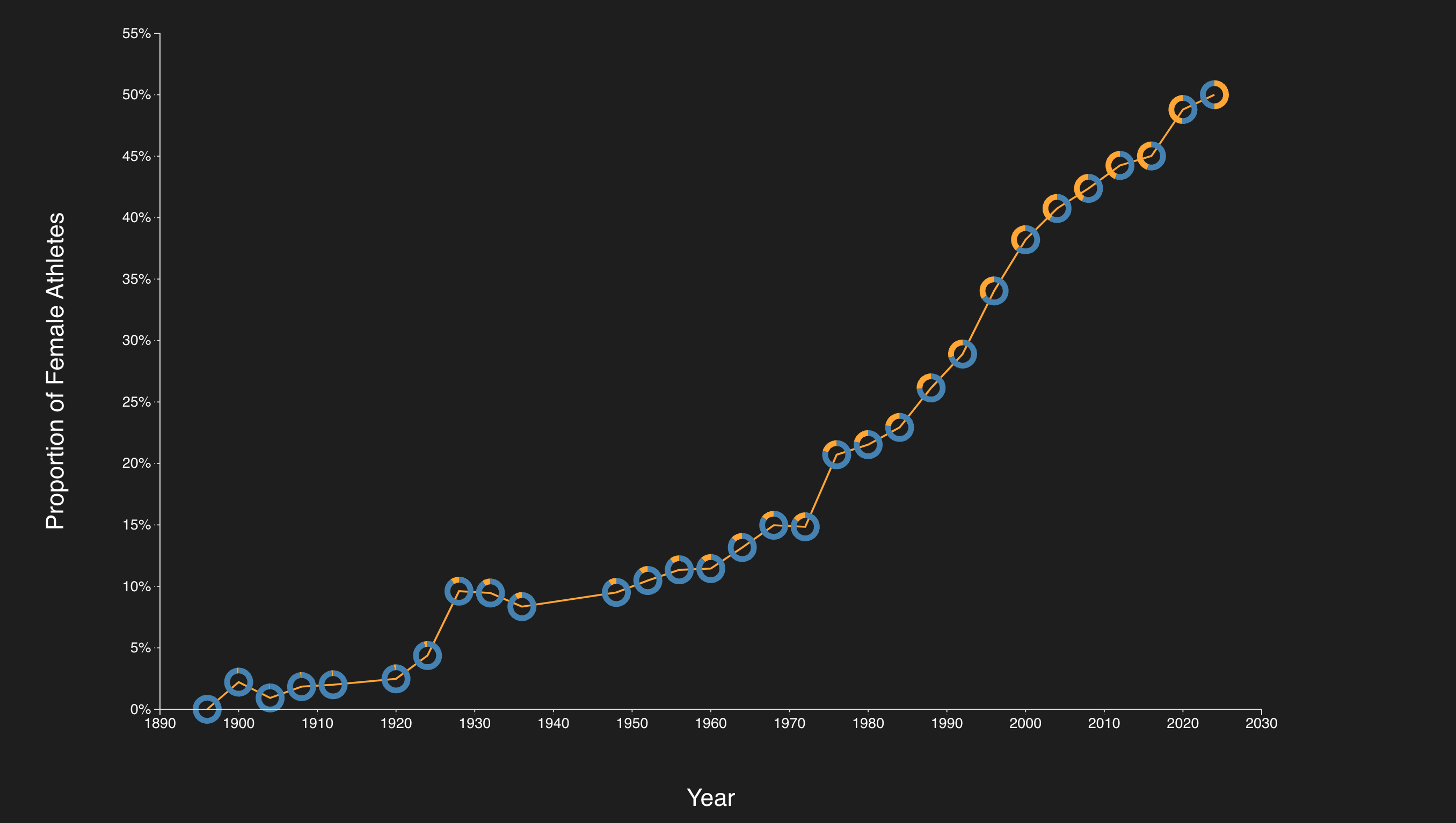
16Olympic donut line
async function build() {
  const W = 960, H = 560;
  const margin = {top: 42, right: 135, bottom: 90, left: 74};
  const w = W - margin.left - margin.right;
  const h = H - margin.top - margin.bottom;
  const svg = d3.select('#chart').append('svg')
    .attr('viewBox', `0 0 ${W} ${H}`).attr('role', 'img')
    .attr('aria-label', "Olympic donut line");
  const plot = svg.append('g')
    .attr('transform', `translate(${margin.left},${margin.top})`);

  const raw = await d3.csv('./examples/02_advanced_charts/datasets/Olympic_Participation_Gender.csv', d3.autoType);
  const data = raw.map(d => ({year: new Date(d.Year, 0, 1), male: d['Male Athlete Count'], female: d['Female Athlete Count']}));
  data.forEach(d => { d.share = d.female / (d.male + d.female); });
  const x = d3.scaleTime().domain(d3.extent(data, d => d.year)).range([0, w]);
  const y = d3.scaleLinear().domain([0, 0.55]).range([h, 0]);
  plot.append('g').attr('transform', `translate(0,${h})`).call(d3.axisBottom(x).ticks(8));
  plot.append('g').call(d3.axisLeft(y).ticks(6).tickFormat(d3.format('.0%')));
  plot.append('path').datum(data).attr('d', d3.line().x(d => x(d.year)).y(d => y(d.share)))
    .attr('fill', 'none').attr('stroke', 'orange').attr('stroke-width', 2);
  const pie = d3.pie().sort(null).value(d => d.count);
  const arc = d3.arc().innerRadius(6).outerRadius(10);
  const donuts = plot.selectAll('.year-donut').data(data).join('g').attr('class', 'year-donut')
    .attr('transform', d => `translate(${x(d.year)},${y(d.share)})`);
  donuts.selectAll('path').data(d => pie([{group: 'Male', count: d.male}, {group: 'Female', count: d.female}]))
    .join('path').attr('d', arc).attr('fill', d => d.data.group === 'Male' ? 'steelblue' : 'orange');
  svg.append('text').attr('x', margin.left).attr('y', 23).text('Female share of Olympic athletes');
  plot.append('text').attr('x', w + 14).attr('y', 25).attr('fill', 'steelblue').text('Male');
  plot.append('text').attr('x', w + 14).attr('y', 50).attr('fill', 'orange').text('Female');
}

build();
Data & source
Lecture 22, slides 72
Exercise solutions
01Horizontal bar chart
async function build() {
  const W = 1280, H = 2100;
  const margin = {"top": 70, "right": 180, "bottom": 60, "left": 350};
  const w = W - margin.left - margin.right;
  const h = H - margin.top - margin.bottom;
  const svg = d3.select('#chart').append('svg')
    .attr('viewBox', [0, 0, W, H].join(' ')).attr('role', 'img')
    .attr('aria-label', "Horizontal bar chart");
  const plot = svg.append('g')
    .attr('transform', 'translate(' + margin.left + ',' + margin.top + ')');

  const raw = await d3.csv('./examples/01_scales_axes_marks/datasets/colleges.csv', d3.autoType);
  const data = raw.filter(d => Number.isFinite(d['SAT Average']) && d.Name)
    .sort((a, b) => d3.descending(a['SAT Average'], b['SAT Average'])).slice(0, 100);
  const x = d3.scaleLinear().domain([0, d3.max(data, d => d['SAT Average'])]).nice().range([0, w]);
  const y = d3.scaleBand().domain(data.map(d => d.Name)).range([0, h]).padding(0.15);
  const color = d3.scaleOrdinal(d3.schemeCategory10).domain(data.map(d => d.Control));
  plot.selectAll('rect').data(data).join('rect')
    .attr('x', 0).attr('y', d => y(d.Name))
    .attr('width', d => x(d['SAT Average'])).attr('height', y.bandwidth())
    .attr('fill', d => color(d.Control))
    .append('title').text(d => d.Name + ': ' + d['SAT Average']);
  plot.append('g').call(d3.axisLeft(y).tickSize(0))
    .selectAll('text').style('font-size', '16px')
    .text(d => d.length > 36 ? d.slice(0, 35) + '…' : d);
  plot.append('g').call(d3.axisTop(x).ticks(6));
  plot.append('g').attr('transform', 'translate(0,' + h + ')').call(d3.axisBottom(x).ticks(6));
  svg.append('text').attr('x', margin.left).attr('y', 24).style('font-size', '20px')
    .text('Top 100 colleges by SAT average');
  const legend = svg.append('g').attr('transform', 'translate(' + (W - 170) + ',70)');
  color.domain().forEach((control, i) => {
    legend.append('rect').attr('y', i * 30).attr('width', 15).attr('height', 15).attr('fill', color(control));
    legend.append('text').attr('x', 22).attr('y', i * 30 + 13).style('font-size', '16px').text(control);
  });
}

build();
Data & source
Lecture 22, slides 22–27
Complete solution using the lecture data. Original source files remain available through Original example.
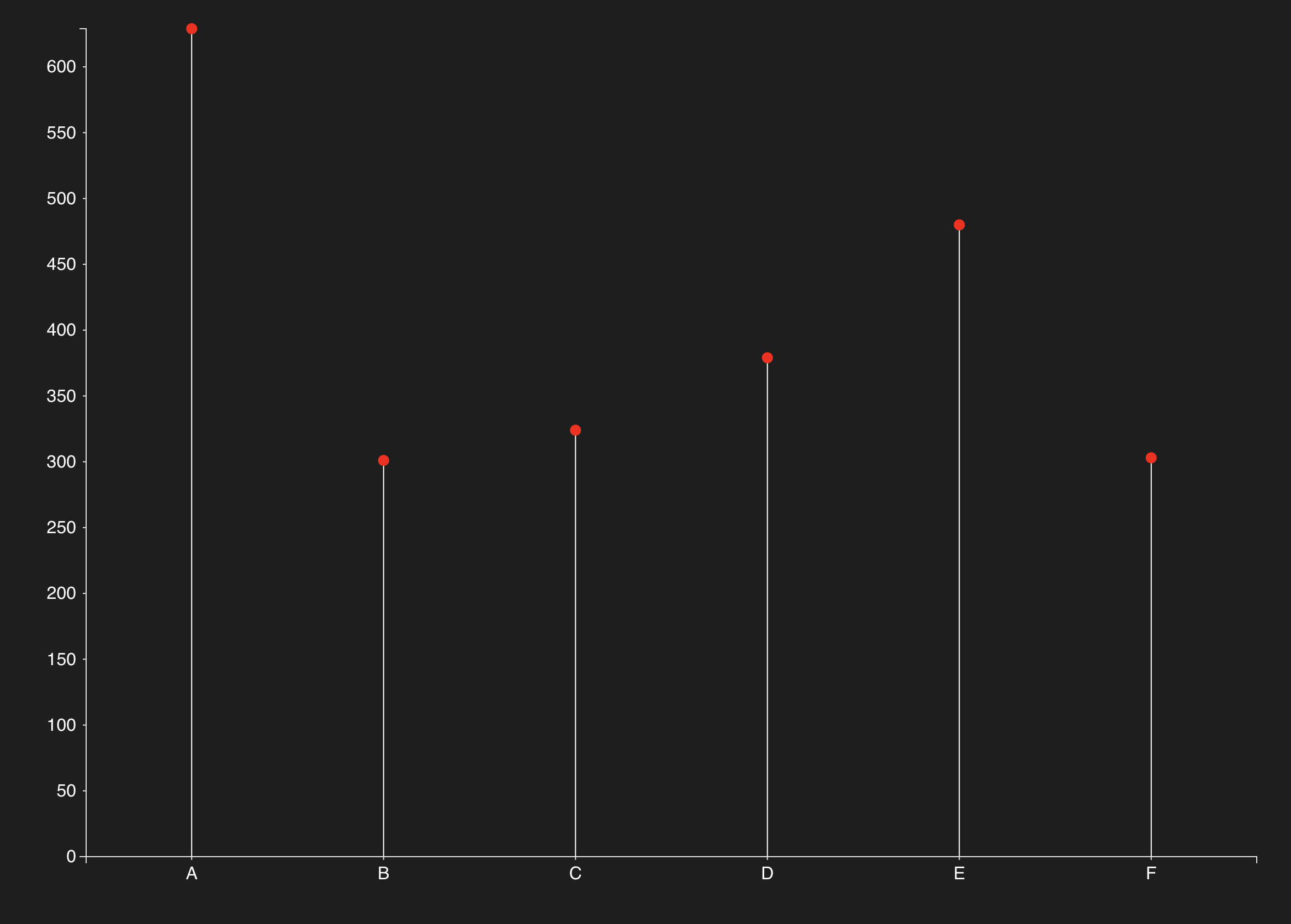
02Lollipop chart
async function build() {
  const W = 960, H = 560;
  const margin = {"top": 42, "right": 135, "bottom": 90, "left": 74};
  const w = W - margin.left - margin.right;
  const h = H - margin.top - margin.bottom;
  const svg = d3.select('#chart').append('svg')
    .attr('viewBox', [0, 0, W, H].join(' ')).attr('role', 'img')
    .attr('aria-label', "Lollipop chart");
  const plot = svg.append('g')
    .attr('transform', 'translate(' + margin.left + ',' + margin.top + ')');

  const data = [
    {Category: 'A', Value: 629}, {Category: 'B', Value: 301},
    {Category: 'C', Value: 324}, {Category: 'D', Value: 379},
    {Category: 'E', Value: 480}, {Category: 'F', Value: 303}
  ];
  const x = d3.scaleBand().domain(data.map(d => d.Category)).range([0, w]).padding(0.45);
  const y = d3.scaleLinear().domain([0, d3.max(data, d => d.Value)]).nice().range([h, 0]);
  plot.selectAll('.stem').data(data).join('line').attr('class', 'stem')
    .attr('x1', d => x(d.Category) + x.bandwidth() / 2)
    .attr('x2', d => x(d.Category) + x.bandwidth() / 2)
    .attr('y1', y(0)).attr('y2', d => y(d.Value))
    .attr('stroke', 'steelblue').attr('stroke-width', 4);
  plot.selectAll('circle').data(data).join('circle')
    .attr('cx', d => x(d.Category) + x.bandwidth() / 2)
    .attr('cy', d => y(d.Value)).attr('r', 10).attr('fill', 'steelblue');
  plot.selectAll('.value').data(data).join('text').attr('class', 'value')
    .attr('x', d => x(d.Category) + x.bandwidth() / 2)
    .attr('y', d => y(d.Value) - 18).attr('text-anchor', 'middle').text(d => d.Value);
  plot.append('g').attr('transform', 'translate(0,' + h + ')').call(d3.axisBottom(x));
  plot.append('g').call(d3.axisLeft(y).ticks(6));
  svg.append('text').attr('x', margin.left + w / 2).attr('y', H - 25)
    .attr('text-anchor', 'middle').text('Category');
  svg.append('text').attr('transform', 'translate(22,' + (H / 2) + ') rotate(-90)')
    .attr('text-anchor', 'middle').text('Value');
}

build();
Data & source
Lecture 22, slides 35
Complete solution using the lecture data. Original source files remain available through Original example.
03Scatterplot
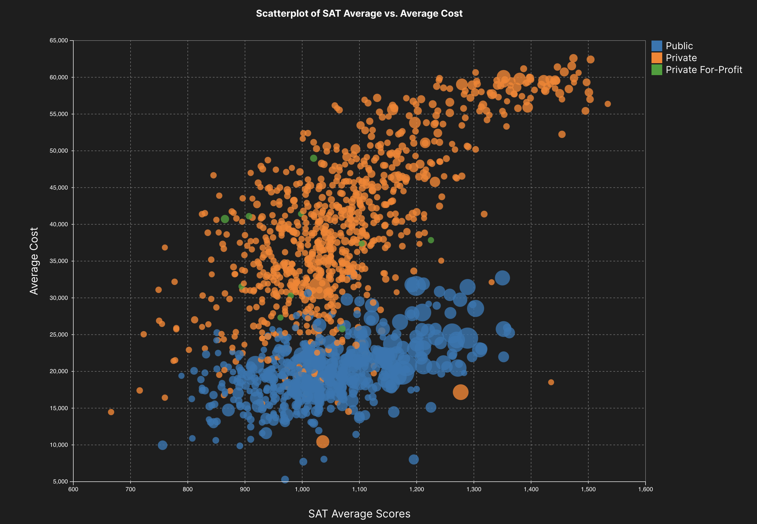
async function build() {
  const W = 960, H = 560;
  const margin = {top: 42, right: 135, bottom: 90, left: 74};
  const w = W - margin.left - margin.right;
  const h = H - margin.top - margin.bottom;
  const svg = d3.select('#chart').append('svg')
    .attr('viewBox', `0 0 ${W} ${H}`).attr('role', 'img')
    .attr('aria-label', "Scatterplot");
  const plot = svg.append('g')
    .attr('transform', `translate(${margin.left},${margin.top})`);

  const raw = await d3.csv('./examples/01_scales_axes_marks/datasets/colleges.csv', d3.autoType);
  const data = raw.filter(d => d['Undergrad Population'] > 0 && d['Average Cost'] > 0 && d['SAT Average'] > 0 && d.Control);
  const x = d3.scaleLinear().domain(d3.extent(data, d => d['SAT Average'])).nice().range([0, w]);
  const y = d3.scaleLinear().domain(d3.extent(data, d => d['Average Cost'])).nice().range([h, 0]);
  const radius = d3.scaleSqrt().domain([0, d3.max(data, d => d['Undergrad Population'])]).range([0, 18]);
  const color = d3.scaleOrdinal(d3.schemeCategory10).domain(data.map(d => d.Control));
  plot.append('g').attr('transform', `translate(0,${h})`)
    .call(d3.axisBottom(x).tickSize(-h).tickFormat('')).attr('opacity', 0.15);
  plot.append('g').call(d3.axisLeft(y).tickSize(-w).tickFormat('')).attr('opacity', 0.15);
  plot.selectAll('.college').data(data).join('circle').attr('class', 'college')
    .attr('cx', d => x(d['SAT Average'])).attr('cy', d => y(d['Average Cost']))
    .attr('r', d => radius(d['Undergrad Population'])).attr('fill', d => color(d.Control)).attr('opacity', 0.6)
    .append('title').text(d => d.Name + ': SAT ' + d['SAT Average'] + ', cost $' + d['Average Cost'] + ', undergraduates ' + d['Undergrad Population']);
  plot.append('g').attr('transform', `translate(0,${h})`).call(d3.axisBottom(x).ticks(6));
  plot.append('g').call(d3.axisLeft(y).ticks(6).tickFormat(d3.format('~s')));
  svg.append('text').attr('x', margin.left + w / 2).attr('y', H - 18).attr('text-anchor', 'middle').text('SAT average');
  svg.append('text').attr('transform', `translate(18,${H / 2}) rotate(-90)`)
    .attr('text-anchor', 'middle').text('Average cost');
  const legend = svg.append('g').attr('transform', `translate(${W - 120},60)`);
  color.domain().forEach((control, i) => {
    legend.append('rect').attr('y', i * 25).attr('width', 12).attr('height', 12).attr('fill', color(control));
    legend.append('text').attr('x', 18).attr('y', i * 25 + 11).text(control);
  });
  legend.append('text').attr('y', 135).text('Undergraduates');
  [10000, 30000, 50000].forEach((value, i) => {
    legend.append('circle').attr('cx', 20).attr('cy', 175 + i * 48)
      .attr('r', radius(value)).attr('fill', 'none').attr('stroke', '#e0e0e0');
    legend.append('text').attr('x', 45).attr('y', 179 + i * 48).text(d3.format('~s')(value));
  });

}

build();
Data & source
Lecture 22, slides 35
Complete solution using the lecture data. Original source files remain available through Original example.
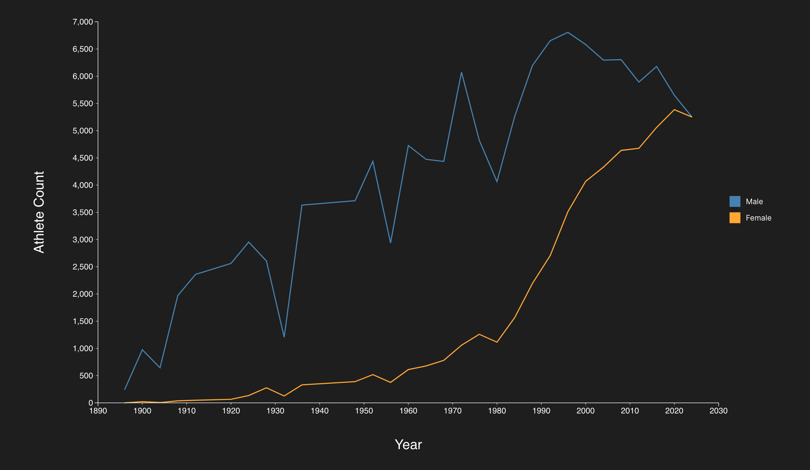
04Olympic participation line chart
async function build() {
  const W = 960, H = 560;
  const margin = {"top": 42, "right": 135, "bottom": 90, "left": 74};
  const w = W - margin.left - margin.right;
  const h = H - margin.top - margin.bottom;
  const svg = d3.select('#chart').append('svg')
    .attr('viewBox', [0, 0, W, H].join(' ')).attr('role', 'img')
    .attr('aria-label', "Olympic participation line chart");
  const plot = svg.append('g')
    .attr('transform', 'translate(' + margin.left + ',' + margin.top + ')');

  const raw = await d3.csv('./examples/02_advanced_charts/datasets/Olympic_Participation_Gender.csv', d3.autoType);
  const data = raw.map(d => ({
    year: new Date(d.Year, 0, 1),
    male: d['Male Athlete Count'],
    female: d['Female Athlete Count']
  })).sort((a, b) => a.year - b.year);
  const x = d3.scaleTime().domain(d3.extent(data, d => d.year)).range([0, w]);
  const y = d3.scaleLinear().domain([0, d3.max(data, d => Math.max(d.male, d.female))]).nice().range([h, 0]);
  const series = [{key: 'male', label: 'Male', color: 'steelblue'}, {key: 'female', label: 'Female', color: 'orange'}];
  series.forEach(({key, label, color}) => {
    const line = d3.line().x(d => x(d.year)).y(d => y(d[key]));
    plot.append('path').datum(data).attr('d', line)
      .attr('fill', 'none').attr('stroke', color).attr('stroke-width', 3);
    plot.selectAll('.point-' + key).data(data).join('circle').attr('class', 'point-' + key)
      .attr('cx', d => x(d.year)).attr('cy', d => y(d[key])).attr('r', 3).attr('fill', color)
      .append('title').text(d => d3.timeFormat('%Y')(d.year) + ' ' + label + ': ' + d[key]);
  });
  plot.append('g').attr('transform', 'translate(0,' + h + ')').call(d3.axisBottom(x).ticks(8));
  plot.append('g').call(d3.axisLeft(y).ticks(6).tickFormat(d3.format('~s')));
  svg.append('text').attr('x', margin.left + w / 2).attr('y', H - 25)
    .attr('text-anchor', 'middle').text('Year');
  svg.append('text').attr('transform', 'translate(22,' + (H / 2) + ') rotate(-90)')
    .attr('text-anchor', 'middle').text('Athlete count');
  const legend = plot.append('g').attr('transform', 'translate(' + (w + 18) + ',20)');
  series.forEach(({label, color}, i) => {
    legend.append('rect').attr('y', i * 28).attr('width', 12).attr('height', 12).attr('fill', color);
    legend.append('text').attr('x', 20).attr('y', i * 28 + 11).text(label);
  });
}

build();
Data & source
Lecture 22, slides 71
Complete solution using the lecture data. Original source files remain available through Original example.
05Donut line
async function build() {
  const W = 960, H = 560;
  const margin = {top: 42, right: 135, bottom: 90, left: 74};
  const w = W - margin.left - margin.right;
  const h = H - margin.top - margin.bottom;
  const svg = d3.select('#chart').append('svg')
    .attr('viewBox', `0 0 ${W} ${H}`).attr('role', 'img')
    .attr('aria-label', "Olympic donut line");
  const plot = svg.append('g')
    .attr('transform', `translate(${margin.left},${margin.top})`);

  const raw = await d3.csv('./examples/02_advanced_charts/datasets/Olympic_Participation_Gender.csv', d3.autoType);
  const data = raw.map(d => ({year: new Date(d.Year, 0, 1), male: d['Male Athlete Count'], female: d['Female Athlete Count']}));
  data.forEach(d => { d.share = d.female / (d.male + d.female); });
  const x = d3.scaleTime().domain(d3.extent(data, d => d.year)).range([0, w]);
  const y = d3.scaleLinear().domain([0, 0.55]).range([h, 0]);
  plot.append('g').attr('transform', `translate(0,${h})`).call(d3.axisBottom(x).ticks(8));
  plot.append('g').call(d3.axisLeft(y).ticks(6).tickFormat(d3.format('.0%')));
  plot.append('path').datum(data).attr('d', d3.line().x(d => x(d.year)).y(d => y(d.share)))
    .attr('fill', 'none').attr('stroke', 'orange').attr('stroke-width', 2);
  const pie = d3.pie().sort(null).value(d => d.count);
  const arc = d3.arc().innerRadius(6).outerRadius(10);
  const donuts = plot.selectAll('.year-donut').data(data).join('g').attr('class', 'year-donut')
    .attr('transform', d => `translate(${x(d.year)},${y(d.share)})`);
  donuts.selectAll('path').data(d => pie([{group: 'Male', count: d.male}, {group: 'Female', count: d.female}]))
    .join('path').attr('d', arc).attr('fill', d => d.data.group === 'Male' ? 'steelblue' : 'orange');
  svg.append('text').attr('x', margin.left).attr('y', 23).text('Female share of Olympic athletes');
  plot.append('text').attr('x', w + 14).attr('y', 25).attr('fill', 'steelblue').text('Male');
  plot.append('text').attr('x', w + 14).attr('y', 50).attr('fill', 'orange').text('Female');
}

build();
Data & source
Lecture 22, slides 72
Complete solution using the lecture data. Original source files remain available through Original example.
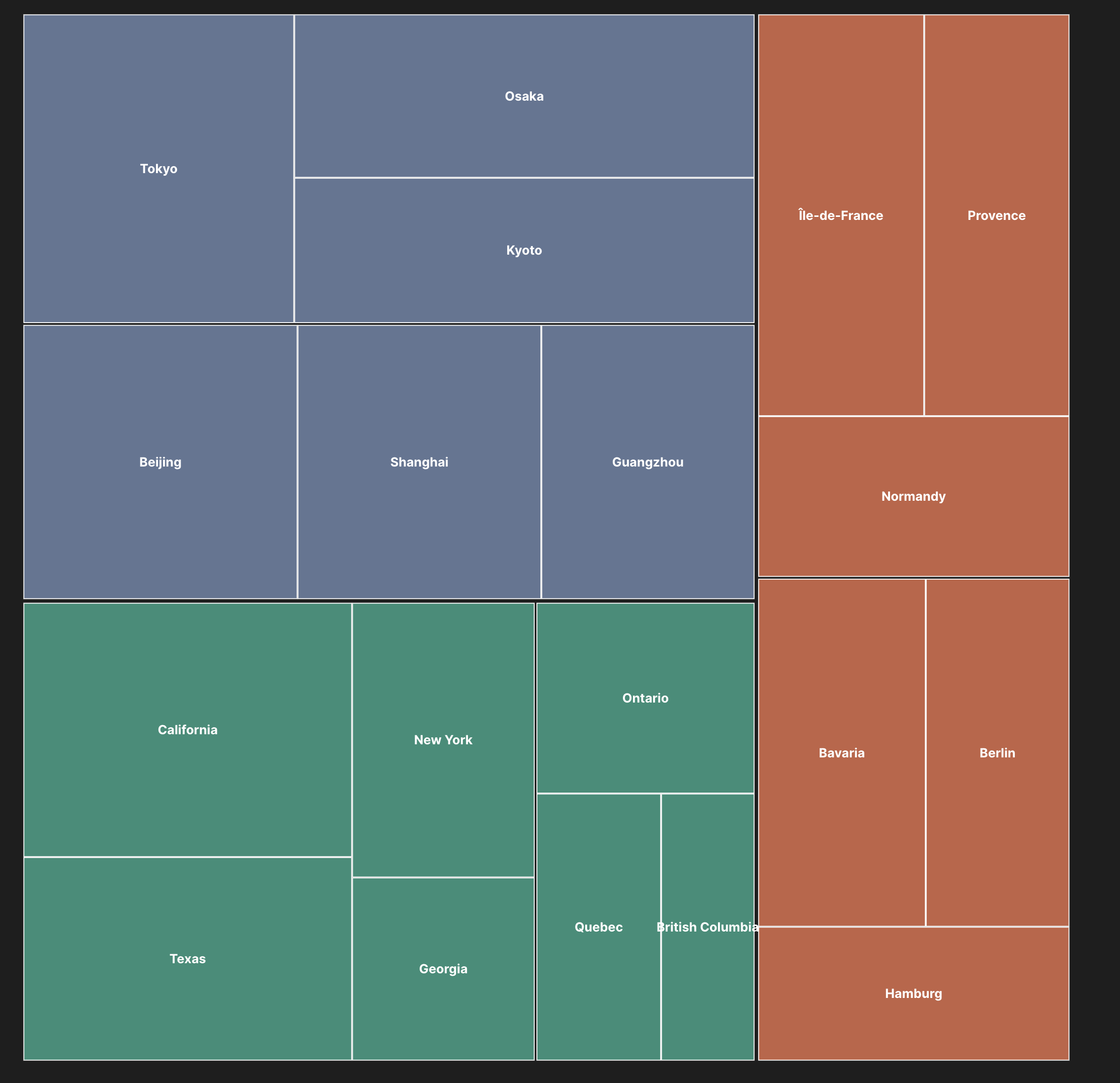
06Treemap
async function build() {
  const W = 1100, H = 760;
  const margin = {"top": 60, "right": 20, "bottom": 20, "left": 20};
  const w = W - margin.left - margin.right;
  const h = H - margin.top - margin.bottom;
  const svg = d3.select('#chart').append('svg')
    .attr('viewBox', [0, 0, W, H].join(' ')).attr('role', 'img')
    .attr('aria-label', "World treemap");
  const plot = svg.append('g')
    .attr('transform', 'translate(' + margin.left + ',' + margin.top + ')');

  const data = {
    "name": "World",
    "children": [
      {
        "name": "North America",
        "children": [
          {
            "name": "USA",
            "children": [
              {
                "name": "California",
                "value": 100
              },
              {
                "name": "Texas",
                "value": 80
              },
              {
                "name": "New York",
                "value": 60
              },
              {
                "name": "Georgia",
                "value": 40
              }
            ]
          },
          {
            "name": "Canada",
            "children": [
              {
                "name": "Ontario",
                "value": 50
              },
              {
                "name": "Quebec",
                "value": 40
              },
              {
                "name": "British Columbia",
                "value": 30
              }
            ]
          }
        ]
      },
      {
        "name": "Europe",
        "children": [
          {
            "name": "Germany",
            "children": [
              {
                "name": "Bavaria",
                "value": 70
              },
              {
                "name": "Berlin",
                "value": 60
              },
              {
                "name": "Hamburg",
                "value": 50
              }
            ]
          },
          {
            "name": "France",
            "children": [
              {
                "name": "Île-de-France",
                "value": 80
              },
              {
                "name": "Provence",
                "value": 70
              },
              {
                "name": "Normandy",
                "value": 60
              }
            ]
          }
        ]
      },
      {
        "name": "Asia",
        "children": [
          {
            "name": "China",
            "children": [
              {
                "name": "Beijing",
                "value": 90
              },
              {
                "name": "Shanghai",
                "value": 80
              },
              {
                "name": "Guangzhou",
                "value": 70
              }
            ]
          },
          {
            "name": "Japan",
            "children": [
              {
                "name": "Tokyo",
                "value": 100
              },
              {
                "name": "Osaka",
                "value": 90
              },
              {
                "name": "Kyoto",
                "value": 80
              }
            ]
          }
        ]
      }
    ]
  };
  const root = d3.hierarchy(data).sum(d => d.value || 0)
    .sort((a, b) => b.value - a.value);
  d3.treemap().size([w, h]).paddingOuter(4).paddingInner(3).round(true)(root);
  const color = d3.scaleOrdinal().domain(data.children.map(d => d.name))
    .range(['#66c2a5', '#fc8d62', '#8da0cb']);
  function continent(d) {
    return d.ancestors().find(a => a.depth === 1).data.name;
  }
  const leaves = plot.selectAll('.region').data(root.leaves()).join('g')
    .attr('class', 'region').attr('transform', d => 'translate(' + d.x0 + ',' + d.y0 + ')');
  leaves.append('rect').attr('width', d => d.x1 - d.x0).attr('height', d => d.y1 - d.y0)
    .attr('fill', d => d3.color(color(continent(d))).darker(d.depth * 0.3))
    .attr('stroke', '#222');
  leaves.append('title').text(d => d.ancestors().reverse().map(a => a.data.name).join(' / ') + ': ' + d.value);
  leaves.append('clipPath').attr('id', (d, i) => 'region-clip-' + i)
    .append('rect').attr('width', d => Math.max(0, d.x1 - d.x0 - 8))
    .attr('height', d => Math.max(0, d.y1 - d.y0 - 8));
  leaves.append('text').attr('clip-path', (d, i) => 'url(#region-clip-' + i + ')')
    .attr('x', 9).attr('y', 23).style('font-size', '16px').text(d => d.data.name);
  leaves.append('text').attr('x', 9).attr('y', 45).style('font-size', '14px')
    .text(d => d.value);
  data.children.forEach((d, i) => {
    const legend = svg.append('g').attr('transform', 'translate(' + (margin.left + i * 190) + ',20)');
    legend.append('rect').attr('width', 14).attr('height', 14).attr('fill', color(d.name));
    legend.append('text').attr('x', 22).attr('y', 12).style('font-size', '16px').text(d.name);
  });
}

build();
Data & source
Lecture 22, slides 73
Complete solution using the lecture data. Original source files remain available through Original example.