Witty Worm Propagation Modeling  ( 09/27/04)

Cliff C. Zou

Most previous worms are "benevolent" worms that do not destroy any resource on compromised computers. "Witty" worm (appeared on March 20, 2004) is the first widely spreading worm that carries a destructive payload.  Shannon and Moore from CAIDA have provided a detailed characterization and analysis of Witty worm based on their comprehensive monitored data [2]. What we are interested, however, is to find out how to model the propagation of Witty worm, especially the decreasing dynamics of Witty worm in the following days after its outbreak. 

Due to the destructive behavior of Witty worm, we classify it as a "destructive worm". From an attacker's perspective, a destructive worm wants to destroy as many computers as possible, thus it should destroy a compromised computer as soon as possible to prevent people from having time to clean the computer; However, destroying a compromised computer might make the computer unable to send out worm packets to infect others, and thus, prevent the worm from spreading out quickly. Therefore, a destructive worm usually needs to make a trade-off between destroying a computer and holding an infected computer for propagation. Witty worm might be the first test worm written by attackers to understand how to design an effective destructive worm.

As analyzed in [2], after sending out 20,000 infection packets, Witty worm writes 65K data to a random point of hard disk on a compromised computer, and then repeats this process until the computer is crashed due to the random destruction of hard disk. Since the destructive data has fixed size 65KB and is written to a random point of hard disk, each hard-disk destructive writing has a very small but constant probability to crash a compromised computer where is determined by the computer's operating system and hard disk size. Suppose a compromised computer is crashed when the worm writes times destructive data, then is a discrete random variable that follows "geometric distribution". 

Define "destruction time" as the time interval from compromising a computer to the crashing of the computer due to Witty's destructive data. Suppose a compromised computer takes a constant time to send out 20,000 infection packets due to its constant network bandwidth, then the destruction time follows geometric distribution, too. Because , the geometric distributed destruction time can be roughly modeled by a continuous "exponential distribution" with a rate . Due to differences in network bandwidth and hard disk volume, different compromised computers have exponential distributed destruction time with different rates ---  we denote the average "destruction rate" as .

Denote as the number of crashed computers due to the destruction of Witty worm. Suppose there are   infectious hosts at time . In the next small time interval , each infected host has the small probability to be crashed --- regardless of how long the host has been infected due to the memoryless property of the exponentially distributed destruction time. Thus on average   infected hosts will be crashed and removed from from time to time (added to ). Taking , based on the uniform-scan worm model in [3], we derive the worm propagation model for Witty worm (which is identical to the Kermack-Mckendrick epidemic model ):

	(1)
	(2)

where is a worm's average scan rate, is the number of IP addresses in the worm's scanning space.

"Internet Motion Sensor" (IMS) in Univ. Michigan has monitored Witty's propagation and provided its  propagation curve in [1]. IMS researchers generously shared the data (in drawing their Witty's propagation figure in [1]) to us, which shows the number of Witty scans per 1000 seconds observed by IMS on three ``/24" blackhole networks --- it can represent the number of infectious hosts in the entire Internet since Witty uniformly scanned the Internet. Researchers in [2] pointed out that Witty had around 110 initially infected hosts and it infected about 12,000 machines, hence in our model, we choose .  since Witty scanned the entire IPv4 space.

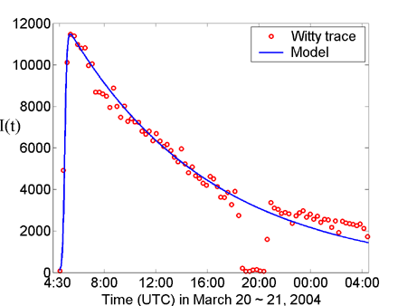
To match the above model with the monitored data, we need to determine the values of and . Fig. 1 shows the monitored data of Witty in red dots, which corresponds to the infectious population as time went on. determines Witty's infection speed, thus we choose per second in order to fit the the growth part of the Witty propagation curve. Since the monitored data is very rough with only four data points in the growth part,   this value of may not be a very accurate estimate. Witty infected almost all vulnerable hosts in the Internet shortly after reached its peak, thus the decay part of Witty's propagation curve shown in Fig. 1 is mainly determined by Equation (2) and the average destructive rate . We choose per second in order to fit the decay dynamics of Witty in the first 24 hours of the worm's outbreak. This value of means that on average a compromised computer would be crashed hours after it was compromised. The infectious population derived from our model is also shown in Fig. 1. This figure shows that our model could model well the propagation of Witty worm.

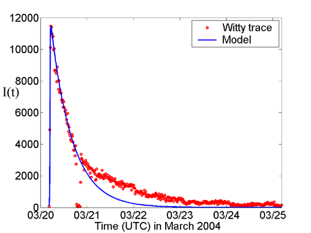
Fig. 1: Infectious population I(t) in the first 24 hours	Fig. 2: Long-time infectious population I(t)

When we consider the monitored worm trace over several days, we find that, as shown in Fig. 2, Witty died out slower than our model predicts. This is because as time went on, Witty infectious computers had a decreasing average destruction rate , not a constant rate as what we use in the above model. Due to hard disk volume and network bandwidth differences, different Witty-infected computers had very different destruction time. After Witty worm infected almost all vulnerable computers in the Internet within one hour [2], compromised computers with larger destruction rates were crashed first, making the remaining infectious computers to have a decreasing average destruction rate as time went on --- the decreasing made the Witty infectious population dropped slower than the above model predicts.

In our Witty propagation modeling, we have not considered other factors that could possibly affect Witty's propagation. For example, some infected computers could have been patched or filtered out by people before they were crashed by Witty worm.  However, if this factor played a major role, then the shown in Fig. 2 should have decreased more quickly in stead of slower than what our model predicts. Therefore, the same as researchers in [2] said, we believe the rapid decay in the number of active infected hosts is primarily caused by Witty's destructive action. 

Acknowledgement:

We gratefully thank researchers in Univ. Michigan "Internet Motion Sensor" for providing us their valuable monitoring data on Witty worm.

Reference:

[1]. University of Michigan. "Internet Motion Sensor". http://ims.eecs.umich.edu/architecture.html

[2]. Colleen Shannon and David Moore. "The Spread of the Witty Worm". http://www.caida.org/analysis/security/witty/

[3]. Cliff C. Zou, Don Towsley, and Weibo Gong. "On the Performance of Internet Worm Scanning Strategies", Umass ECE Technical Report TR-03-CSE-07, November, 2003.