The following web page was written in January 2002. Since then, we have conducted further research on this topic and published a paper in ICCCN'04:

  Cliff C. Zou, Don Towsley, and Weibo Gong. "Email Worm Modeling and Defense," 13th International Conference on Computer Communications and Networks (ICCCN'04), October 11-13, Chicago, 2004 (Best Paper Nominee, extended from previous Technical Report TR-03-CSE-04).

      Email virus and worm propagation simulation  (Jan 2002)

1. Brief introduction.

2. Mesh structure topology modeling and simulation.

3. Power law topology modeling and simulation.

4. A simple explanation of various spreading cycle effect on virus&worm propagation.

1.  Brief Introduction

Email virus is one of the major Internet security problems nowadays. Usually a virus email has an attachment file that contains copy of the virus. The virus hides the attachment file’s executable property by forging it to be any type of files, like image, word document, etc. When an email user clicks on this attachment, the virus program will be activated and infect the local computer. Then it will send itself as attachment to all email addresses in the user’s email address book.

Though this technique is an old virus spreading method, it is still a very effective way and widely used by current viruses and worms. It has some advantages that make it attractive to hackers:

1. Email virus does not require any security holes in computer OS or software (as long as to those viruses that require clicking of users).
2. Almost everyone who uses computer nowadays is using email service.
3. Emails are private information like post office letters. So it’s hard to allow checking content of each email to detect virus before end user receives the email.
4. A large part of computer users have little or no knowledge of email virus and trust all emails he/her received.

There are very little paper published on virus propagation simulation[1]. During summer 2001 Code Red worm booming period, some people wrote brief simulation of code red propagation, but with no depth research. 

Here we try to thoroughly study the behavior of email virus propagation. We use simulation instead of mathematic analysis to approach it because of the complexity of users’ behavior and their email address books’ relationship.

2. Mesh structure modeling and Simulation

For email virus simulation, there is no physical topology issue since all emails are end-to-end communication. But at the same time, there is a logical topology of email address book relationship. For example, all email addresses in a user’s address book will be his friends’, or his job related email addresses. So in our model, all topology are email address logical topology.

For simplicity, currently we use two-dimensional mesh structure for the email address logical topology. Each node on this mesh network represent one computer with a single email address associated with. The distance between two nodes represents their friendship. In this way, a node email address book will be likely to only contain those nodes in the nearby area.  In our model, we give a local-preferred parameter to adjust this relationship and to check the effect of this relationship. “Localization probability” is the portion of email addresses that are in the local area; the other part of email addresses is random chosen from the entire nodes space. “Localization range” defines the local area size.

In our model, we try to consider the user’s checking email, clicking email attachment and email address book statistical properties. It is reasonable to assume that:

1. A user’s checking email time interval is exponential distributed.
2. Each user’s checking email rate, clicking e-mail’s probability, email address book size are fixed, but considering all users behaviors, they are normally distributed.

And we also assume that all nodes are vulnerable to this email virus. At initial state, only 2 randomly chosen nodes are infected with the virus.

In our experiment results, we use emailList(20, 10) to represent normal distribution of email address book, which has average 20 email addresses and variance of 10´10. “clickProb” is the clicking probability of nodes when it has virus emails. “checkTime” is the checking email time interval of a user.

Experiment 1:  reinfection vs. non-reinfection.

 The following graph shows the difference between two situations. One is that each infected node allows reinfection and will send out virus copies to other nodes whenever virus email clicked. The other one is non-reinfection case that each infected node will send out virus copies only once. Because a node’s email address book is fixed. Sending out virus copies to the same nodes again and again does not increase infection very much (though it increases the possibility a little bit).

It’s clear to see that allowing reinfection will increase spreading speed and dramatically increase the number of infected computers. 

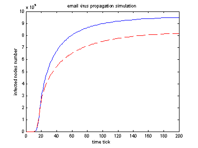Red dashed line: non-reinfection.   Blue solid line: allow reinfection.      Parameters: (nodes 1000* 1000)   (2 initial infected node)     emailList (20, 15),   checkTime(20,15),   clickProb(0.5,0.3),   Localization probability  = 0.7,   Localization range=10

Note: In re-infection experiment, though email list number is fixed but which node to infect is randomly selected each time, so re-infection case is not realistic. We can think of it more likely to be the code red worm’s spreading processes.

Experiment 2:  local preferred infection vs. random infection ( non-reinfection case).

Because email addresses have logical relationship, we want to know how it affects email virus propagation. The following graph shows the effect of local preference infection compared with random infection where there is no logical relationship between users’ email address books.

It’s clear to see that random infection will have faster spreading speed than strictly local preference infection case. But if there is a little bit random relationship in user’s email address book, the virus propagation will behave just like random relationship case.

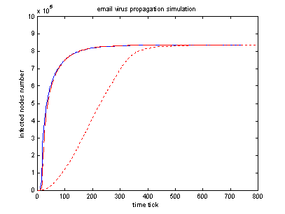Blue solid line: random infection Red dashed line: local infection.            (Localization probability  = 0.95). Red dotted line: strictly local infection            (Localization probability  = 1.0).   Parameters: (nodes = 1000 * 1000) (2 initial infected node ) emailList (20, 15), checkTime(20,15), clickProb(0.5, 0.3), Localization range=10 (For local preferred infection)

Experiment 3: large size email address book vs. small size email address book:

Another aspect we are interested in is the effect of user’s email address book size. The following graph shows that email address book size plays a very important role in email virus propagation. Large number of email addresses in user’s address book will dramatically increase email virus spreading speed as well as total number of infected computers.

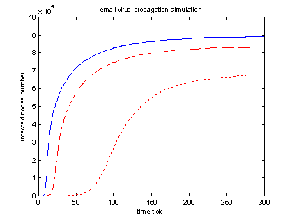Blue solid lines:   emailList = ( 60, 40) Red dashed line:  emailList = ( 20, 15) Red dotted line:   emailList =  ( 5, 3)   Parameters:  ( nodes = 1000 * 1000), (2 initial infected node)   checkTime(20,15), clickProb(0.5, 0.3),  Localization part =0.95,  Localization range=10

3. Power law topology modeling and simulation.

In the previous model, mesh structure is too simple to capture users' email addresses relationship. It's preferred to generate a network topology that each node represents a user, and the links in and out this node represent email  address reference of this user. For example, out links mean that those nodes connected to this node are email users' whose email addresses are in this user's email address book. 

But it's difficult to model email address relationship. Unlike Internet topology, we can not collect information and data of email address books because they are all personal private information.  We can not do this investigation without user's fully acceptance. So currently we can only "guess" such kind of relationship. We think "Power Law" maybe suitable for email address book relationship. We know that city population, Internet connection are power law and we think it's reasonable to think that each user's email address book is built step by step as city population evolution. The more communicative a person is, the more email addresses he might to add to his large email address book. 

Except for the power law topology, all other assumptions are the same as mesh structure modeling.  In the power law topology simulation, virus propagation is strictly hop by hop along links between nodes.

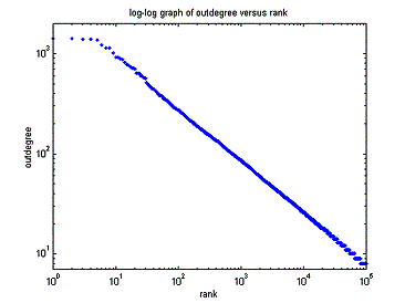
There are a lot power law topology generators currently available in academic world. In order to generate the power law topology suitable for us, we used BRITE [2] power law topology generator since we can modify the least link number of added new nodes in this generator.

I. Non-immunization case.

Experiment 1:  reinfection vs. non-reinfection.

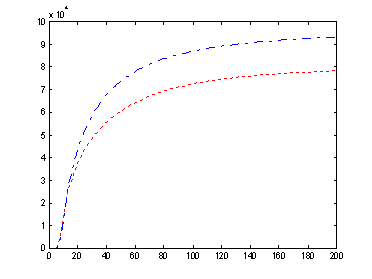
2 random infected nodes, non-reinfection case.  100,000 nodes, 8 base-degree.

Blue dash-dot line:  allow reinfection.                                              Red dotted line:  non-reinfection	Power law property of the topology generated by BRITE  ( 100,000 nodes, 8 base-degree)

Experiment 2:  most connected vs. least connected initial infected nodes (reinfection case, Base degree = 8).

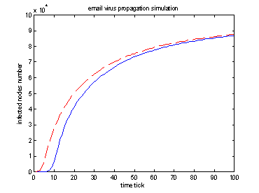Red dashed line: 2 most connected initial infected nodes. (degree = 1418, 1419 ). Blue solid line: 2 least connected initial infected nodes. (degree = 8, 8 ).

100,000 nodes degree distribution: 

 Experiment 3:  most connected vs. least connected initial infected nodes (Base degree = 2)

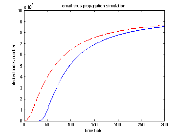Red dashed line: 2 most connected initial infected nodes ( degree = 794, 723). Blue solid line: 2 least connected initial infected nodes ( degree = 2, 2 ).

II. Partial immunization effect

 Experiment 4:  most connected vs. least connected nodes immunization ( Base degree = 8)

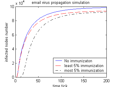Blue solid line: no immunization. Red dashed line:     5 % least connected nodes immunization Black dashed line:    5% most connected nodes immunization.   (2 most connected initial infected nodes)

Experiment 5:  most connected vs. least connected nodes immunization ( Base degree = 2)

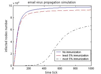Blue solid line: no immunization. Red dashed line:     5 % least connected nodes immunization Black dashed line:    5% most connected nodes immunization.   (2 most connected initial infected nodes)

Conclusion: When network are not densely connected, selective immunization on high degree nodes have significant effect to slow down email propagation.

Experiment 6:  effect of checking time statistic

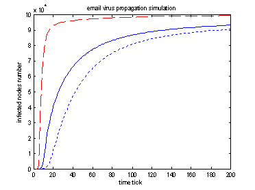Topology base node degree: 8 Red dashed line: checkTime(3  ,  0.1) Blue solid line:   checkTime(20,  15 ) Blue dotted line: checkTime(20,  0.1)

Conclusion: for solid and dotted lines, they have equal average checking time, so spreading speed is determined by those faster infection nodes, not average spreading value.

4. A simple explanation of various spreading cycle effect on virus&worm propagation.

( Explanation about experiment 6 )

 Question: Why various checking time case’s speed is much faster than fixed checking time case’s though they have equal average checking time?

 Answer: Because before the fixed time case gives birth to next generation, the various time case has already given birth to SEVERAL generations although each generation’s population is small. ( Snowball effect).

 Proof: A simplified proof model:

Suppose there is no reinfection, each node will infect fixed number C healthy nodes when it actives. Now we have two situations, the first one every virus copy has fixed active period, T; the second one every virus has exponential distributed active period with mean value of T. So these two models have the same average propagation activation period.

Let  be the infected node number of case one at time ;  be the number of case two. For case one, it is a deterministic equation:

,   Initial status                                                     (1)

 For case two, it has stochastic process in it but we can use mean value analysis to write the following equation: (Note that exponential distribution has memoryless property)

  ,  Initial status                                                     (2)

Since for exponential distribution, the cumulative distribution function:

                                                                       (3)

Solving these two iterative equations, we have:

                                                           (4)

 From the problem, we know that these parameters are required as: ; Integer variable ; Integer variable

 From equation (4), only when C=1, T=2 then  will be bigger than . For all other cases,  will always be much bigger than , which means that the various checking time case’s speed will always be faster than fixed checking time case.

 Here we used exponential distribution model because of its memoryless property. For other statistic distribution, we cannot get an equation like (2). 

Reference:

[1]. Wang, C., J.C. Knight, M. Elder. On Viral Propagation and the Effect of Immunization, 16th ACM Annual Computer Applications Conference, New Orleans, LA (December 2000).

[2]. Alberto Medina, Anukool Lakhina, Ibrahim Matta, and John Byers. BRITE: An Approach to Universal Topology Generation. In Proceedings of the International Workshop on Modeling, Analysis and Simulation of Computer and Telecommunications Systems- MASCOTS '01, Cincinnati, Ohio, August 2001.